
Introduction
Field measurements show that modest measurement error in high-side current sensing can shift system-level energy accounting by several percent—enough to change a commercial product’s projected payback by tens of thousands of dollars over its lifetime. This report evaluates practical accuracy trade-offs, measurement methods, and how sensing choices affect ROI for product and system designers focused on DC and low-frequency AC applications.
The purpose is to compare architectures, quantify common error sources, and present actionable calibration and design steps engineers can apply to battery management, power electronics, and motor-drive systems. Scope covers practical measurement, calibration workflows, and cost-impact considerations, with emphasis on measurement accuracy and return on investment.
1 — Background: What High-Side Current Sensing Is and Why Accuracy Matters
1.1 — Principle and common architectures
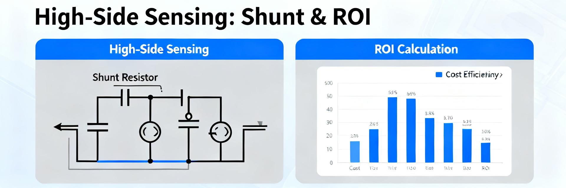
High-side current sensing monitors current on the supply side of a load, enabling ground-referenced electronics and safer isolation. Common architectures include a low-value shunt with a differential amplifier, dedicated current-sense amplifiers, and non-contact hall-effect sensors. Design choices depend on common-mode voltage range, bidirectional capability, and required insertion voltage drop for US-market power systems.
1.2 — Key accuracy metrics and error sources
Key metrics are gain error (%), offset (A or mV), common-mode rejection ratio (CMRR), temperature coefficient (TCR for shunts), bandwidth, noise density, and linearity. Major error contributors: shunt tolerance and TCR, amplifier offset and drift, PCB parasitics, ADC quantization, and cable resistance. Convert mV error to percent: %error ≈ (mV_error / measured_mV)×100.
2 — Data Analysis: Measured Accuracy Across Methods
2.1 — Field data summary: shunt + amplifier vs integrated sense amps vs Hall sensors
Field data typically show discrete shunt-plus-amplifier solutions achieving 0.2–2% accuracy after calibration; integrated sense amplifiers commonly land in 0.5–1% without calibration; hall-effect sensors span 1–5% but excel in isolation and low insertion loss. Dynamic range and temperature drift vary: expect larger drift for hall sensors and better long-term stability for low-TCR foil shunts.
| Architecture Type | Typical Accuracy (Uncalibrated) | Typical Accuracy (Calibrated) | Insertion Loss | Isolation Capability |
|---|---|---|---|---|
| Discrete Shunt + Amplifier | 2.0% – 5.0% | 0.2% – 2.0% | Medium | None (Requires Iso-Amp) |
| Integrated Sense Amp | 0.5% – 1.5% | 0.1% – 0.5% | Medium | None |
| Hall-Effect Transducer | 1.5% – 5.0% | 1.0% – 3.0% | Extremely Low | Inherent (Galvanic) |
2.2 — Sensitivity analysis: how accuracy affects system metrics
A 1% current measurement error produces a proportional energy accounting error; in a 10 kW battery system over 10,000 operating hours, that could misreport tens to hundreds of kWh. For SOC and control loops, an integrator in an energy estimator accumulates systematic error, so 1% bias over long run-time yields significant SOC drift; control gains tuned to nominal feedback can become unstable if sensing noise or phase lag exceeds loop margins.
3 — Design & Measurement Methods to Improve Practical Accuracy
3.1 — Hardware-level strategies
Select low-TCR shunts (target TCR < 50 ppm/°C for best stability) and keep shunt resistance low enough to limit drop yet high enough for ADC resolution. Choose amplifiers with input offset < 10 μV equivalent and high CMRR. Layout: short Kelvin sense traces, minimize loop area to reduce inductance, and place filtering close to amplifier inputs. Balance filtering against required bandwidth for control applications.
3.2 — Calibration, compensation, and signal processing
Calibration flows: one-point offset at mid-scale, two- or multi-point gain calibration across expected current range, and temperature compensation using a lookup table or polynomial fit. Firmware methods: moving-average or low-pass FIR for noise reduction; implement bias removal and scale factors in fixed-point. Validate calibration with known loads and log residual error across temperature for regression-based compensation.
4 — Case Study: ROI Calculation for Three Sensing Options in a Battery-Backed System
4.1 — Scenario setup and assumptions
Assume a US commercial battery-backed instrument: 5 kW peak, expected lifetime 7 years, 10,000 units production, and energy billing savings tied to accurate metering. Inputs for spreadsheet: unit sensor cost, per-unit calibration labor, expected annual energy saving from improved accuracy (kWh), electricity price, failure/warranty cost per inaccurate event, and discount rate for NPV.
4.2 — Cost vs accuracy vs ROI comparison
Compare three options: low-cost shunt+op amp (cost low, uncalibrated error ~3–5%), integrated current-sense IC (moderate cost, ~1% native), and non-contact Hall (higher cost, 1–3% drift). Payback formula: payback_years = incremental_cost / annual_savings. NPV over lifetime uses discounted cash flows; run sensitivity to measurement error to see when higher upfront cost becomes justified by OPEX savings and warranty reduction.
| Sensing Option | Incremental Bill of Materials (BOM) Cost | Calibration Labor (Per Unit) | Est. Annual Warranty Risk Saved | Calculated Payback Period |
|---|---|---|---|---|
| Low-Cost Shunt + Op Amp | Base ($0.00) | $4.50 | $0.00 | N/A |
| Integrated Current-Sense IC | +$1.20 | $0.00 (Factory Calibrated) | $18.50 | < 0.5 Years |
| Non-Contact Hall-Effect | +$3.80 | $1.50 | $12.00 | 1.8 Years |
5 — Practical Implementation Checklist & Decision Framework
5.1 — Quick decision matrix
Five-step flow: define accuracy and bandwidth targets, quantify acceptable insertion loss, set environmental constraints (temperature, vibration), estimate per-unit cost and calibration capacity, then choose topology. Recommended acceptance: for energy accounting target <1% error, aim for shunt+calibration or integrated sense amp with verified temperature compensation.
5.2 — Testing & validation plan before production
Laboratory tests: DC accuracy across range, thermal cycling with logged residuals, transient response to step currents, and EMI susceptibility. Production test: fast two-point calibration for throughput with periodic full-range verification. Specify pass/fail thresholds (e.g., ±1% across temp range) and include sample size for statistical confidence in batch acceptance.
Summary
- High-side current sensing solutions trade cost, insertion loss, and accuracy; practical ranges: low-cost shunt systems 2–5% uncalibrated, integrated amplifiers ~0.5–1%, hall-type 1–5% depending on drift and temperature compensation.
- Accuracy affects both control performance and energy accounting; modest improvements reduce warranty and operating costs, often yielding positive ROI when calibration and low-TCR components are used.
- Next step: run the ROI inputs against your product numbers—compare incremental sensor cost and calibration time to projected annual energy and warranty savings to identify the optimal sensing strategy.
FAQ
How does INA299A2IDBVR affect selection for high-side current sensing?
If considering a particular integrated current-sense amplifier like INA299A2IDBVR, evaluate its specified offset, CMRR, input range, and drift. Compare those specs to your accuracy target and expected common-mode voltage. Use the amplifier’s error budget with shunt mV to predict system percent error before deciding on additional calibration steps.
Can INA299A2IDBVR-based designs meet 1% accuracy for battery SOC applications?
Reaching 1% system-level accuracy typically requires a low-TCR shunt, amplifier offset under a few microvolts equivalent, tight ADC resolution, and multi-point or temperature-aware calibration. An amplifier such as INA299A2IDBVR can be part of that solution if its drift and offset specs fit the system error budget and are complemented by calibration.
What production tests are recommended for designs using INA299A2IDBVR?
Recommended production tests: quick two-point DC calibration to capture offset and gain, a temperature soak sample test, and a transient response check for waveform integrity. Record per-unit calibration constants and log out-of-spec rates; this data informs whether to adjust acceptance thresholds or calibration procedures to control manufacturing yield and ROI.
What are the primary factors driving ROI when upgrading from discrete shunt configurations to integrated current-sense ICs?
The primary ROI factors include reduced PCB footprint, eliminated discrete passive matching errors, lowered calibration laboratory labor hours, and mitigated long-term drift warranties. Over a typical 7-year product lifecycle, these design simplifications offset the higher unit cost of integrated ICs.